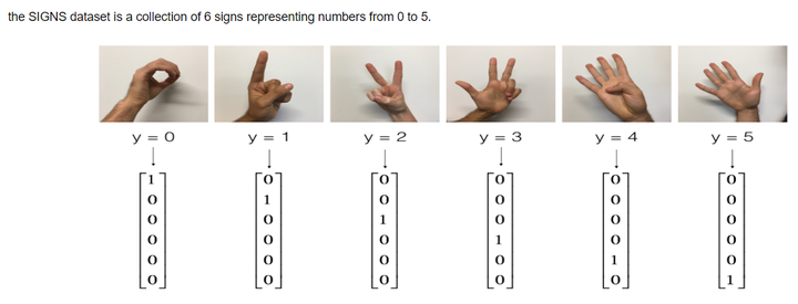
编程作业-卷积基础2

1 | import math |
1 | X_train_orig, Y_train_orig, X_test_orig, Y_test_orig, classes = load_dataset() |
1 | # Example of a picture |
y = 5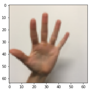
改变数据形状,转化为独热编码
1 | X_train = X_train_orig/255. |
number of training examples = 1080
number of test examples = 120
X_train shape: (1080, 64, 64, 3)
Y_train shape: (1080, 6)
X_test shape: (120, 64, 64, 3)
Y_test shape: (120, 6)
1 | def creat_placeholders(n_H0, n_W0, n_C0, n_y): |
1 | def initialize_parameters(): |
In TensorFlow, there are built-in functions that carry out the convolution steps for you.
tf.nn.conv2d(X,W1, strides = [1,s,s,1], padding = ‘SAME’): given an input $X$ and a group of filters $W1$, this function convolves $W1$’s filters on X. The third input ([1,f,f,1]) represents the strides for each dimension of the input (m, n_H_prev, n_W_prev, n_C_prev). You can read the full documentation here
tf.nn.max_pool(A, ksize = [1,f,f,1], strides = [1,s,s,1], padding = ‘SAME’): given an input A, this function uses a window of size (f, f) and strides of size (s, s) to carry out max pooling over each window. You can read the full documentation here
tf.nn.relu(Z1): computes the elementwise ReLU of Z1 (which can be any shape). You can read the full documentation here.
tf.contrib.layers.flatten(P): given an input P, this function flattens each example into a 1D vector it while maintaining the batch-size. It returns a flattened tensor with shape [batch_size, k]. You can read the full documentation here.
tf.contrib.layers.fully_connected(F, num_outputs): given a the flattened input F, it returns the output computed using a fully connected layer. You can read the full documentation here.
In the last function above (tf.contrib.layers.fully_connected), the fully connected layer automatically initializes weights in the graph and keeps on training them as you train the model. Hence, you did not need to initialize those weights when initializing the parameters.
Implement the forward_propagation function below to build the following model: CONV2D -> RELU -> MAXPOOL -> CONV2D -> RELU -> MAXPOOL -> FLATTEN -> FULLYCONNECTED. You should use the functions above.
In detail, we will use the following parameters for all the steps:
- Conv2D: stride 1, padding is “SAME”
- ReLU
- Max pool: Use an 8 by 8 filter size and an 8 by 8 stride, padding is “SAME”
- Conv2D: stride 1, padding is “SAME”
- ReLU
- Max pool: Use a 4 by 4 filter size and a 4 by 4 stride, padding is “SAME”
- Flatten the previous output.
- FULLYCONNECTED (FC) layer: Apply a fully connected layer without an non-linear activation function. Do not call the softmax here. This will result in 6 neurons in the output layer, which then get passed later to a softmax. In TensorFlow, the softmax and cost function are lumped together into a single function, which you’ll call in a different function when computing the cost.
向前传播
1 | def forward_propagation(X, parameters): |
计算损失
- tf.nn.softmax_cross_entropy_with_logits(logits = Z3, labels = Y): computes the softmax entropy loss. This function both computes the softmax activation function as well as the resulting loss. You can check the full documentation here.
- tf.reduce_mean: computes the mean of elements across dimensions of a tensor. Use this to sum the losses over all the examples to get the overall cost. You can check the full documentation here.
1 | def compute_cost(Z3, Y): |
1 | tf.reset_default_graph() |
cost = 4.664871 | def model(X_train, Y_train, X_test, Y_test, learning_rate = 0.009, |
1 | _, _, parameters = model(X_train, Y_train, X_test, Y_test) |
Cost after epoch 0: 1.921332
Cost after epoch 5: 1.904156
Cost after epoch 10: 1.904309
Cost after epoch 15: 1.904477
Cost after epoch 20: 1.901876
Cost after epoch 25: 1.784094
Cost after epoch 30: 1.687814
Cost after epoch 35: 1.617914
Cost after epoch 40: 1.588563
Cost after epoch 45: 1.564673
Cost after epoch 50: 1.551985
Cost after epoch 55: 1.512204
Cost after epoch 60: 1.488463
Cost after epoch 65: 1.368796
Cost after epoch 70: 1.281402
Cost after epoch 75: 1.209459
Cost after epoch 80: 1.120872
Cost after epoch 85: 1.098565
Cost after epoch 90: 1.046483
Cost after epoch 95: 1.007478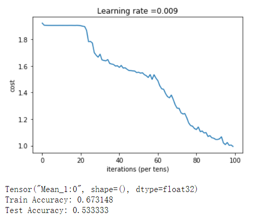
转载请注明来源,欢迎对文章中的引用来源进行考证,欢迎指出任何有错误或不够清晰的表达。可以在下面评论区评论,也可以邮件至 2470290795@qq.com
文章标题:编程作业-卷积基础2
文章字数:1.2k
本文作者:runze
发布时间:2020-03-02, 22:41:17
最后更新:2020-03-02, 22:51:00
原始链接:http://yoursite.com/2020/03/02/%E5%90%B4%E6%81%A9%E8%BE%BE%20%E6%B7%B1%E5%BA%A6%E5%AD%A6%E4%B9%A0/04%E5%8D%B7%E7%A7%AF%E7%A5%9E%E7%BB%8F%E7%BD%91%E7%BB%9C/%E7%BC%96%E7%A8%8B%E4%BD%9C%E4%B8%9A-%E5%8D%B7%E7%A7%AF%E5%9F%BA%E7%A1%802/版权声明: "署名-非商用-相同方式共享 4.0" 转载请保留原文链接及作者。

